In 2014, Ian Goodfellow introduced the Generative Adversarial Network (GAN) as a novel technique to generate samples from a target probability distribution from which a data set is already available. The GAN works by an adversarial process, in which two units, called the Generator and the Discriminator, are pit against each other in a mini-max game-theoretic setting, with the generator creating samples of “fake” data and the discriminator distinguishing between real and fake data. At each step, the generator updates its samples in a way that it may “fool” the discriminator into classifying them as genuine. After a sufficient number of steps, if the data set provided is large enough and the architectures in both units are suitable, the samples generated by the generator start resembling the real data, and improve with each step of the game (up to a saturating point).

Goodfellow proved that under ideal circumstances (infinite real data), the game converges, with the generator generating samples indistinguishable from the real samples, and the discriminator completely confused between the two classes of data. Though the game seldom converges in practical situations, GANs and their modifications have been shown to be efficient data-generating models, with their samples resembling reality with sufficient accuracy.

The DCGAN (Deep Convolutional GAN) developed by Alec Radford, Luke Metz and Soumith Chintala (2016) has been used extensively for the generation of images. In this model, each of the generator and the discriminator is a deep convolutional neural network (CNN). Several architectures, additional features, and modifications have been incorporated into the DCGAN, and it has been found to perform well on most popular image data sets.

In this article, we will experiment with two versions of the DCGAN architecture, and two different versions of a data set comprising images of different species of flowers. The first data set (flowers-17) comprises only 1360 images of 17 varieties of flowers, while the second data set (flowers-102) comprises 8189 images of 102 varieties of flowers. Thus, apart from empirically studying the effects of tuning hyper-parameters and modifying the architecture, we will also witness the level of difference brought about in performance by expanding the training data set. Here is the link to download both data sets: http://www.robots.ox.ac.uk/~vgg/data/flowers/

The files are downloaded as .tgz tar files, and need to be unloaded as images.n (> 💡 Note: In modern Python, it’s safer to use with tarfile.open(...) as tar: instead of manually opening and closing the tar file. It ensures automatic cleanup even if errors occur.) This is done using the tarfile library of Python. The images are then read as pixel arrays using the OpenCV2 library, and are reshaped and combined into a single tensor that can easily be fed into the neural networks. A sample code for this process follows:

import tarfile
import collections
import os
import cv2
import numpy as np

# Extract the image files from the downloaded tar file
# Here, we use the larger dataset with 102 flower types.
# The same code works for the 17-label dataset, by merely changing the file/variable names.

k = tarfile.open('102flowers.tgz')
k.extractall()
k.close()

# The images are now extracted into the working directory in .jpg form.
# We write the image file names into a list and then into a text file named "flowers102" for future use.

files = list()
DirectoryIndex = collections.namedtuple('DirectoryIndex', ['root', 'dirs', 'files'])

for file_name in DirectoryIndex(*next(os.walk('.\\working_folder'))).files:
    # insert the path of the working directory in the quotes
    if file_name.endswith(".jpg"):
        files.append(file_name)

# Create a blank text file named flowers102 in the working directory
textf  = open('flowers102.txt','w')
for file in files:
    textf.write(file + "\n")
textf.close()

# Now we extract the digital forms (pixel representations) of all the images.

line_file = 0
flowers = np.zeros((len(files), 32, 32, 3))  # the tensor which will hold the digital forms of the images

l = 0
for line in open("flowers102.txt"):  # loop over all entries of the text file
    line = line.strip('\n')
    line_file = line
    img = cv2.imread(line_file, cv2.IMREAD_COLOR)
    img1 = cv2.resize(img, (32, 32))              # resize the image to have 32 rows and 32 columns
#We resize to 32×32 for speed and simplicity. For higher-quality results, modern DCGANs often use image sizes of 64×64 or larger.
    img2 = np.asarray(img1, dtype='float32')      # convert to numpy array
    flowers[l] = img2                             # populate the tensor with pixel values of each image
    l += 1  # l ranges from 0 to 8188

print(flowers.shape)

Note that for the code to work, the required blank text file “flowers102.txt” must be created in the working directory.

Part 3: First Experiments with Architecture-2 (Flowers-17)

Once the images have been prepared in the form of tensors, we may start experimenting with the architectures. First, we take a brief overview of the two architectures. Clearly, the major differences are the absence of single-side label smoothing and batch discrimination in the second architecture, and of dropout in the first. The generator of the first architecture is also a layer deeper than that of the second.

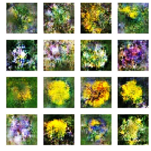
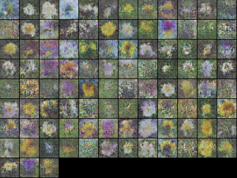
We begin by looking at the results of architecture 2 on the 17-label dataset. Since the original data set contains a majority of yellow and purple flowers, the GAN has fallen into mode collapse, having generated only these colours. Following are the results at the end of the 10000th epoch.

Compare this to the results when only a selected batch of the data set was used as input. In such a case, more colours are obtained in the output images.

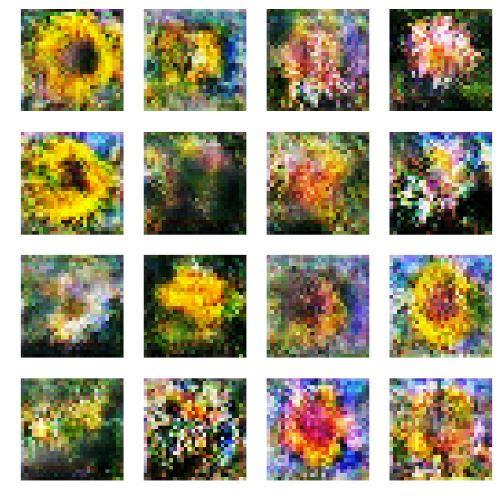
Even though the data set is reduced in size in the second case, the images are more or less the same in quality. In fact, the resulting images are not drastically different even if the input data set is set to comprise of only flowers of a single label, as is done below:

This shows that the GAN is picking up only a very small subset of features from the real data, and falling into mode collapse. This is why increasing the data set size is not improving its performance. Thus, architecture-2 requires modifications to solve this problem. Batch discrimination and single-sided label smoothing are commonly prescribed solutions to this problem, and are used in architecture-1.

Part 4: Mode Collapse, Grayscale Inputs, and Learning Rate Tweaks

One may expect the picture quality to go up if grayscale images are input, because the problem seems simplified with the number of input parameters being reduced threefold (fewer parameters, thus making learning easier). However, the picture quality does not improve in this case. While grayscale images reduce input dimensionality, they also strip out color variation, which is a rich source of learning for GANs. So the “simplification” doesn’t always help — and expressivity may suffer.

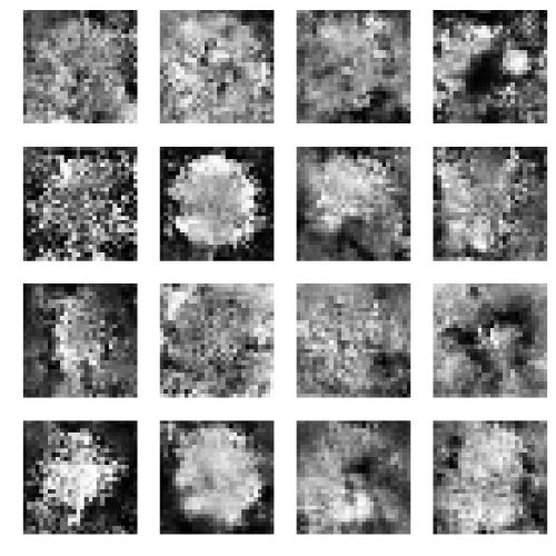
All the above results are when the learning rates of the discriminator and generator are set to be equal. When the learning rate of the discriminator is doubled, as is sometimes done in GANs, the mode collapse problem becomes worse, and sometimes only images of a single colour (yellow or purple) are generated. On the other hand, this improves the sharpness slightly for grayscale images.

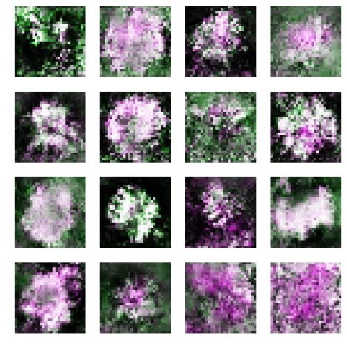
Now moving to architecture-1, the image below demonstrates that this DCGAN out-performs the one discussed above in terms of clarity of the flowers as well as variety:

The above images were generated using a batch size of 16. It is found that increasing the batch size (to 32) as well as reducing it (to 8) both deteriorate the resulting images. Note that the model has mixed features of different varieties of flowers to generate new ones. There are some flowers generated that have blends of colours (half the flower is purple-ish, smoothly blending into the other half, which is white).

Also note that the mode collapse problem has drastically reduced, with white flowers now being generated in equal proportion to the yellow and purple ones. This is the result of using batch discrimination and single-sided label smoothing.

One possible reason why architecture-1 generates relatively smoother and less pixelated images is its use of double strides rather than upsampling along with transposed convolution, as used in architecture-2. Another possibility is the existence of an extra transposed convolutional layer in the generator. If dropout is introduced into the first architecture, its performance deteriorates greatly, with the generated images having blurred-out patches in several regions.

Part 5: Parameter Tweaks and Scaling to the Flowers-102 Dataset

A number of different experiments were conducted: changing the label smoothing from (0.1, 0.9) to (0.2, 0.9), doubling the weightage of batch discrimination and removing it completely, changing the optimizers and noise types (between Gaussian and uniform), etc. In most cases, small changes were observed in the results, but these were nominal.

We now use architecture-1 on the larger flowers-102 dataset. Probably since this dataset is far larger, a batch size of 16 does not give the best results. The images improve with increasing batch size, at least till a size of 64:

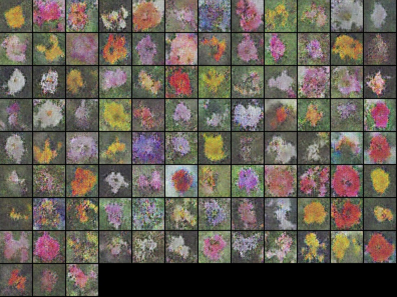
The above result is obtained after running the DCGAN (architecture-1) for 20,000 epochs, though the results are more or less the same after the 15,000th epoch. Throughout, we are measuring the “goodness” of our results only by assessing them visually. Another method to do this is by looking at the discriminator’s predictions on the real data, and the generated images. In the ideal scenario, where the game has reached convergence, both these numbers should be 0.5. This convergence is, of course, not achieved in reality. Modern GAN evaluation often uses metrics like Fréchet Inception Distance (FID) or Inception Score to quantify image quality. We stick to visual inspection here due to its simplicity and interpretability.

However, at the end of 20,000 epochs, the numbers are reasonable, ranging from 0.1 to 0.9 for architecture-1. For architecture-2, the results are much nearer to 1, since the dataset (flowers-17) is smaller, the generated images are not near enough to the real ones, and there is no label smoothing: thus, the discriminator is highly confident of its real/fake classification.

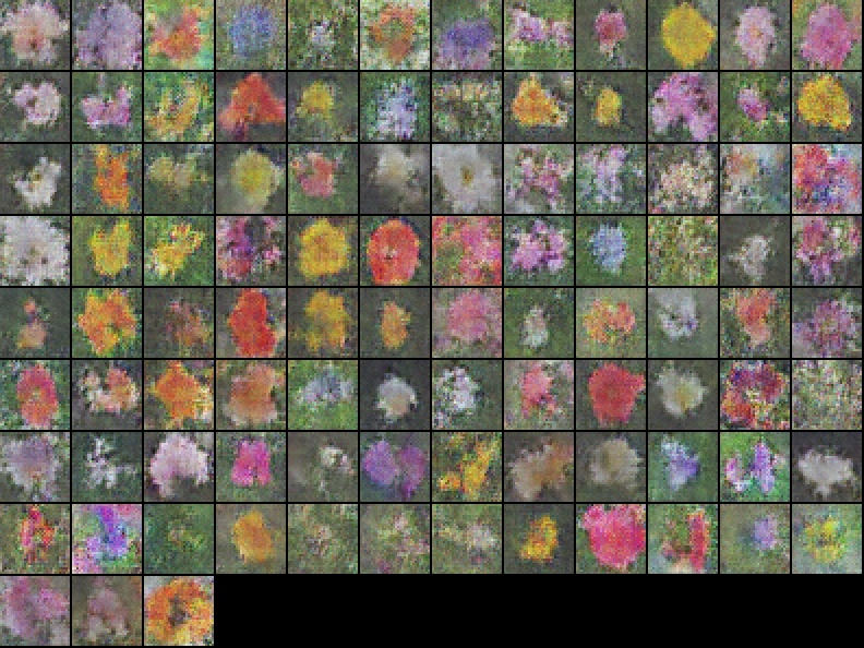
The images may further be sharpened by adding a random Gaussian noise to the results of the generator, with the intensity decreasing with increasing epochs. The final results are:

The entire codes for the entire architectures and procedure, including unloading and pre-processing the data can be found at:

https://github.com/simrantinani/Experimenting-with-DCGANs-using-the-flowers-dataset