Perceptrons from Scratch: A Starting Point for Machine Learning -

Introduction

The Perceptron Learning Algorithm is one of the simplest machine learning algorithms and a crucial building block of more complex machine learning and deep learning models. A neural network is, in fact, known as a multi-layer perceptron (MLP), because (of course) it is composed of several layers of perceptrons stacked together. Apart from providing a glimpse into the working of a neural network, an understanding of a perceptron’s working is essential for a beginner to grasp the most fundamental concepts of machine learning. A simple modification of this algorithm is termed the Pocket Learning Algorithm. In this article, we will build the simple perceptron and the pocket learning algorithm from a scratch, and check their performance in classifying points in the 2-dimensional Euclidean plane into two halves. Minimal expertise in coding in R is assumed, and most of the code is self-explanatory.

Defining the Training Space and Target Function

First define the limits of the space to work in during training: let $(x_1, y_1)$ and $(x_2, y_2)$ be the coordinates defining this rectangular subspace of the $XY$ plane. I have taken them to be $(-2,-2)$ and $(2,2)$ respectively. Note that “<-” is the assignment operator in R.

x_1 <- (-2)
y_1 <- (-2)
x_2 <- 2
y_2 <- 2

We now wish to define the target function, which is, in our case, a straight line. We let this line be defined as the line passing through two random points in the training domain (the subspace defined by (x_1, y_1) and (x_2, y_2)).

x <-  runif(2, min = x_1, max = x_2)
y <- runif(2, min = y_1, max = y_2)
fit <- (lm(y~x))

We now define our target function by extracting the coefficients of the fit.

t <- summary(fit)$coefficients[,1]
f <- function(x){
  t[2]*x + t[1] #(general line equation: y = slope*x + intercept)
}

Creating the Training Dataset

Now we define the number of points from the training domain to be taken in the training set. I have taken this number to be $1000$. This number $N$ and the limits $x_1$, $x_2$, $y_1$, $y_2$ may be experimented with later. Then, we create and populate separate matrices for the training data points and their classification labels based on the line defined by function $f$.

N <- 1000 # Number of data points in the training set
A <- matrix(ncol=N, nrow=2) # N random points of the space
b <- matrix(ncol=N, nrow=1) # labels of the points in A: i.e. which                                                    #                             side of the line they lie on

for(i in 1:N){
  A[, i] <- c(runif(2, min = x_1, max = x_2)) # random entries in       #                                              the training domain
  b[1, i] <- sign(A[2, i] - f(A[1, i])) # whether the point in A[,i]                                           #                                         lies above or below the 
}

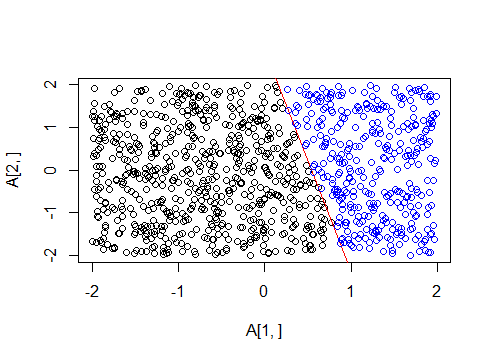
# Visualization
plot(A[1, ], A[2, ]) 
abline(fit,col="red") 
k=which(b==1)
points(A[1,k], A[2,k], col="blue") # points above the line are        #                                    labelled 1

An example plot showing linearly separable data — An example of the plots obtained

Perceptron Algorithm: Initialization and Updates

The plot provides a neat visualization of what we have done so far. We have $1000$ points and a line predefined in a plane. Every point above the line is labelled 1 and every point below the line is labelled $-1$. Now assume that the functional form of the line is taken away from us, and we are only left with the points and their labels. We want a function $g$ that can approximate the classification of the line we had in the best way, on the entire XY plane. That is, we want a function that will separate the plane in a way as similar as possible to the original line, given only these $1000$ training points.

We do this by beginning with a random vector of coefficients, $w$, which defines our hypothesized line $g,$ checking its classification on the given points, and iteratively updating it in a way such that at each iteration, it does a better job at the classification of the points. Here, we have started with $w$ as a vector of zeroes.

# Initialization

w <- rep(0,3) # initial values in the weight vector
g <- function(z){ # function g will attempt to approximate f            
 t(w) %*% z
}

Weight Update Rule and Intuition

At each step, a random point out of the $1000$ available training points is selected, and the hypothesis function defined by the vector $w$ is evaluated on the point. If the point $(x, y)$ with label $p$ is in the training set (here, $p \in {1, -1}$), and turns out to be classified wrongly by $w$ (i.e., $w$ predicts its label to be $-p$), $w$ is updated so that its new value equals $w + (x, y) \cdot p$. We do this for $2000$ steps (in general, $2 \cdot N$) to ensure that updating is done with a sufficient number of distinct training points.

At each step, this new $w$ is more likely to classify the same point correctly, because its prediction on the same point is now

$$ \text{sign}\left((w + (x, y) \cdot p)^T \cdot (x, y)\right) = \text{sign}\left(w^T \cdot (x, y) + p \cdot (x, y)^T \cdot (x, y)\right) $$

where $T$ denotes the transpose of a vector and $\cdot$ denotes matrix multiplication. For someone unfamiliar with linear algebra, the notation simply means that the weights are being multiplied element-wise to the components of the point, and the sign of that product is giving the side of the line on which the point lies.

When $p = 1$, $\text{sign}(w^T \cdot (x, y))$ must be $-1$, since the point is assumed to be misclassified by $w$ (i.e., $g$). Adding a positive quantity, $p \cdot (x, y)^T \cdot (x, y)$, to it makes it more likely for the prediction by the new $w$ (thus $g$) to be correct.

When this process is repeated a sufficient number of times, a good percent of the training set points end up correctly classified, and the resulting weights/hypothesis function are then used to classify every point on the plane.

Also note that in the above discussion, $w$ is assumed to be a two-dimensional vector. However, $w$ needs an additional $1$ appended to its front, to account for the constant term in a 2D line’s equation $(a \cdot x + b \cdot y + c)$. This has been done in the code.

Pocket Learning Algorithm

Above, we have defined the Perceptron Learning algorithm. The Pocket Learning algorithm is a simple modification. Since the algorithm proceeds by updating the weights using a single point at each step, the overall accuracy on the training set might go down in a single update. In the pocket algorithm, instead of using the classification function obtained at the end of all iterations, one simultaneously calculates the training accuracy at each step, and stores the most accurate hypothesis function obtained from each past step. At the end, the hypothesis is the best possible that could be obtained from the training set with this algorithm.

w_pocket <- w # Pocket (best) weight vector
training_accuracy<-0 # at each iteration, this will be added to
pocket_accuracy<-0 # the best achievable accuracy
i_pocket<-0 # index at which pocket accuracy is achieved

i <- 1

while(i < 2*N+1){
  j = sample(1:N, 1)
  if((sign(g(c(1, A[, j]))) == b[1, j]) == 0){ 
    # update the weight vector at each misclassified point
    w <- w + b[1, j]*c(1, A[, j])
  }
  training_accuracy<-c(training_accuracy,0)
  for(k in 1:N){
    if(sign(g(c(1, A[,k ]))) == b[, k]){
      training_accuracy[length(training_accuracy)] <- training_accuracy[length(training_accuracy)] + 1/N
    }
  }
  if(tail(training_accuracy,1)>max(head(training_accuracy,-1))){
    w_pocket<-w
    i_pocket<-i
    pocket_accuracy<- tail(training_accuracy,1)
  }
  i = i + 1
}

final_training_accuracy <- tail(training_accuracy,1) 
# training accuracy at the last iteration

Evaluating Test Accuracy

We have calculated both training accuracies. It is now time to calculate test accuracies. Since the test set is a continuous space, we cannot evaluate the exact classification accuracy, we can only estimate it by taking a large random sample of discrete points from the entire space. Here, we take 100,000 such points. We also want the domain to be much larger than the training domain, and so we take the test limits to be 100 multiplied by the old training limits.

# Preparing a larger sample data set to approximate test accuracy

S <- matrix(ncol=(N*100), nrow=2) # matrix with 10000 random entries

for(v in 1:(N*100)){
 S[, v] <- c(runif(2, min = min(x1,y1)*100, max = max(x2,y2)*100)) 
}

# Simple Perceptron

test_accuracy <-0
v <- 1
while(v <= (ncol(S))){ 
 if(sign(g(c(1, S[, v]))) == sign(S[, v][2] — f(S[, v][1]))){
 test_accuracy <- test_accuracy + 1/ncol(S)
 }
 v <- v + 1
}

# Pocket Learning Algorithm

pocket_test_accuracy <-0
v <- 1
g_pocket <- function(z){ # function g_pocket multiplies by w_pocket
 t(w_pocket) %*% z
}

while(v <= (ncol(S))){ 
 if(sign(g_pocket(c(1, S[, v]))) == sign(S[, v][2] — f(S[, v][1]))){
 pocket_test_accuracy <- pocket_test_accuracy + 1/ncol(S)
 }
 v <- v + 1
}

All the calculations are now complete, and we may display our results in terms of percentages.

print(i_pocket) # at i_pocket, training accuracy stopped increasing
print(final_training_accuracy*100) # Perceptron training accuracy
print(pocket_accuracy*100) # Pocket training accuracy
print(test_accuracy*100) # Perceptron test accuracy
print(pocket_test_accuracy*100) # Pocket test accuracy

Experimental Results

In many cases, the pocket and perceptron algorithms yield the same results. This corresponds to the case where the last iteration step yields the highest accuracy among all. In others, the perceptron yields lower training and test results than the pocket algorithm. Examples of both these types of results yielded by a run of the entire code follows.

# Run 1
> print(i_pocket) 
528
> print(final_training_accuracy*100) 
96
> print(pocket_accuracy*100) 
98.4
> print(test_accuracy*100) 
95.24
> print(pocket_test_accuracy*100) 
97.82

# Run 2
> print(i_pocket) 
[1] 1091
> print(final_training_accuracy*100) 
[1] 99.9
> print(pocket_accuracy*100) 
[1] 99.9
> print(test_accuracy*100) 
[1] 95.523
> print(pocket_test_accuracy*100) 
[1] 99.523

Note that the relation between the training and testing accuracy values depends on how the test domain and number of test points are chosen. If the test set is scaled to maintain the same density of points (i.e. using the same scaling factor for number of points as for the dimensions of the subspace), as was done in the above code, the result will be as expected, i.e. the training accuracy will be higher than the testing accuracy.

However, if the test domain has a smaller density of points, the same line is likely to have many more correct classifications, thus making the test accuracy higher than the training accuracy. For instance, when the test domain was scaled to 1000 times the training domain, but the number of points increased only 100-fold, here were the results:

> print(i_pocket) 
[1] 1543
> print(final_training_accuracy*100) 
[1] 99.5
> print(pocket_accuracy*100)  
[1] 99.7
> print(test_accuracy*100) 
[1] 99.991
> print(pocket_test_accuracy*100) 
[1] 99.976

On the other hand, if the density of points is increased, i.e. the number of points is increased by a larger factor than the dimensions of the test domain, the training accuracy will always be higher, and the difference between the training accuracy and test accuracy becomes larger than in the case of same density. For instance, when the test domain was scaled to only 10 times the training domain, but the number of points increased 100-fold, here were the results:

> print(i_pocket) 
[1] 2000
> print(final_training_accuracy*100) 
[1] 99.8
> print(pocket_accuracy*100)  
[1] 99.8
> print(test_accuracy*100) 
[1] 99.689
> print(pocket_test_accuracy*100)
[1] 99.689

Of course, the exact same numbers will not be replicated since the code works with random values and no seed has been set. Clearly, plenty of experimentation can be done with different domains, different densities, different training and test sizes, and different initialization of w. The entire article has dealt with only two dimensions, but the same algorithms can be generalized to any number of dimensions, and will indeed prove useful where the data is known to be linearly separable. One of the best ways to learn about something from within is to build it from scratch. Having done that, perhaps one is now convinced that there is a lot more to the humble perceptron than one had earlier thought.